This post describes the aerodynamics around airfoils in a way that I haven’t seen presented elsewhere. At a past job, I developed blade shapes for turbomachines and it would sit and wonder why certain changes that I made to the blade shape changed the flowfield and pressure field the way that they did. Ultimately, I was interested in the net torque on the blades, much of which was due to the pressure field. Whereas CFD was the tool I was using to determine the final torque loads, I needed a fast and intuitive way to determine, directionally, what changes would lead me where I was trying to go with the blade performance. Thus, the thought process described below was born.

The logic of this working model is as follows:
- The fluid packet in Figure 1 is flowing from left to right and is following the streamline as shown. To a first approximation, a semi-experienced flow analyst could draw moderately reasonable streamlines for a body without doing an analysis or test, I think.
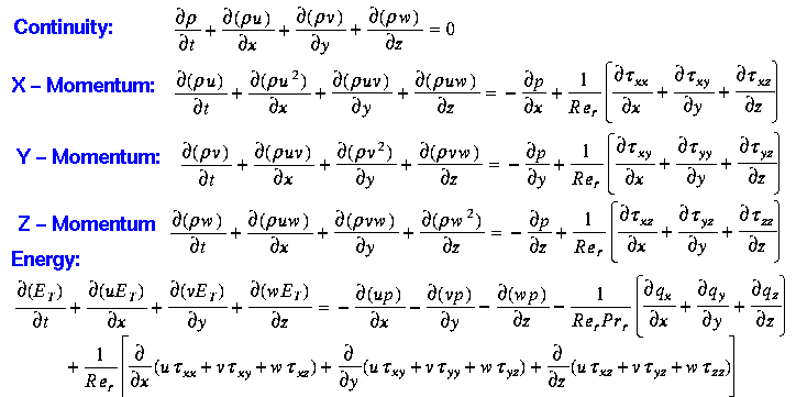
- Bends in the streamlines come from a net force on the fluid particles which are following the streamline path, which is considered to be not changing with time. Why would a fluid particle speed up, slow down, or turn? Where do we get a net load on a fluid particle? The flow equations shown below tell us that fluids can get a net force from a pressure gradient and also from shear stress. In particular, the primary thing driving a bend in a streamline is a pressure gradient; relatively higher pressure is on the outer radius side of the bend and relatively lower pressure is towards the center of the bend radius circle.
- Looking at the streamlines, and understanding the pressure gradients that we can read from them, we can figure out what kind of pressure we will end up observing on the surface of the body – the thing that gives us the majority of the net load on the profile. Figures 2, 3, and 4 below illustrate the pressure field that we can infer from the streamlines there. It’s a simple matter of identifying relatively higher static pressures on the outer radius of a bend and a lower static pressure on the inner radius.
- Note that the only thing we can infer from the streamline bends are the local, relative pressure gradient on the fluid particles tracing out the streamline. For example, in Figure 4, we can infer that there is a lower pressure near the surface of the body, which increases as we move (normally) away from it, and this gradient is responsible for turning the flow along the blade profile. But what we can’t say is whether the pressure gradient exists because the static pressure near the wall of the blade has decreased, or because the static pressure further away from the wall has increased. All we know is that there is a gradient to turn the flow. I get a little stuck here, but I believe there must be a least-energy rule that we can call upon to say that the airfoil produces local static pressure changes (rather than changing the static pressure of the entire atmosphere!).
This framework ends up being useful and meshes with the high level control volume analysis of airfoils (the airfoil imparts a net momentum to the flow in the downward direction to generate upwards-directed lift), but with a more detailed description of the physics which makes it useful for doing design work and developing an intuition for how design changes will play out. Let’s look at this example applied to an airfoil.
An example airfoil (it’s asymmetric, and also at a slightly positive angle-of-attack) is shown in Figure 2 below, with accompanying eyeballed streamlines. Are the streamlines unreasonable looking? They seem OK to me; and again, just about anybody could take a good guess as to what these look like just upon looking at them. We just need to apply the thought process given above to these streamlines and see what kind of pressure field we end up with. Figure 3 takes the first step and illustrates that the particular streamline which is highlighted turns at different radii in different locations. As expected based on normal physics, for an air packet moving at a given speed, tighter radii turns require a higher net load to be carried out. As noted above, the net load driving the air packet in these circles is a pressure gradient normal to the flow direction.

At the level of the gas dynamics, you can just imagine a packet of air moving along a surface, but the surface is effectively moving away from the air packet as it moves along, thus generating a lower static pressure. I plan to give a more thorough description in a future post about this.


Pressure: The Dimension Coupler
Vector field plots and contour plots in two dimensions can be confusing to look at at times, because there can be action in the direction into the page which may need to be accounted for in order to understand the flow behavior. In fact, all else equal, there is flow into or out of the page which is happening. Although the momentum equations share many variables between the x, y, and z direction equations, pressure is really the one to pay attention to when developing an intuition about flow. I think it is useful to think of static pressure as the main dimensional coupler at work here.
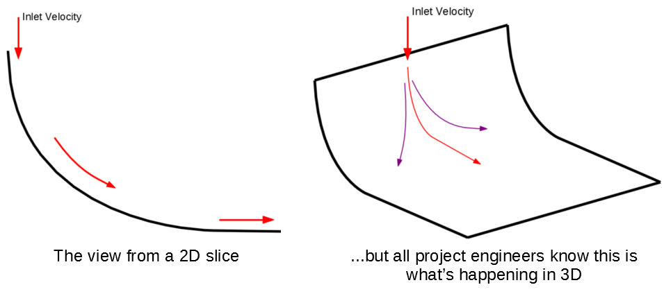
At least, for the source terms, pressure is the one which commonly has the largest impact on the overall flow field. An example of this effect is shown in the figure below. The figure at left is what you would see in a 2D cut – and that’s what we see in the airfoil streamline figures above – but it is not the full story. Whereas the primary effect we see in this section is the the flow turns 90 degrees between the inlet and outlet, there is a notable secondary component here. The increase in static pressure at the wall, which is generated in order to turn the flow translates into a net pressure gradient in the direction into the page as well. In the figure at right, the purple lines are illustrations of the streamlines which arise just because of this directional coupling effect of pressure. Of course, this effect is happening whenever you see a 2D figure of flow turning (whether intended or not), and is part of the explanation for wingtip vortices.
Using the Model
This way of thinking about the flow around an airfoil (or any body) allows one to make useful predictions about how changes to the geometry and operating conditions will impact loads on the body, and to develop an intuition about the static pressure field around the body. This is a working model (whereas almost all other descriptions of airfoil aerodynamics don’t address the static pressure generation mechanism with enough detail or correctness to make predictions) because it allows us to understand what happens when we apply design or operating condition changes to the situation. What happens if the air velocity over the airfoil increases? To the extent that the streamlines stay the same and the flow attached, the pressure gradients have to increase to allow faster air packets to traverse the same streamlines – more exaggerated pressure gradients lead to greater lift. What happens if we curve the airfoil a bit more and turn the flow more (for example, decrease r3 in the Figure 4 above)? The pressure gradient must get steeper in order to turn an air packet on this tighter radius for the same speed, and thus we get more lift again. This breaks down when, at some point, you ask the flow to make a turn that it is unable to do, and you get separated flow. But even then, the same kind of streamline analysis is useful in understanding whats happening.
Updated August 17, 2021