Generative AI is going to change the world, and change how we do product design. Many vague AI-as-a-panacea promises have been made, and many checks cashed with the promise of essentially easy access to unlimited, perfect knowledge. I have heard it described as a question of when rather than if. Bold claims. How can we come to an understanding of what generative AI is capable of, what it’s role may be, and what the trajectory may look like over time?
There are things that computer models are excellent at and which our brains are not. In a sentence, I would say that computers are materially different in terms of processing and/or finding trends in large sets of data. As noted elsewhere, I have used neural network models to process information contained in fluid flow simulation results. The neural network was trained on the data set and was serving as a useful surrogate model in no time at all. If my brain would have been able to do this, it would have taken me many months, at a minimum. This is a clear case where the neural network was serving a uniquely valuable function; basically serving as a data-processing extension of my brain. In the future, could a hyper-logical AI have guided the design process as well as carried out the mechanics of the work – basically, could it have replaced me?
Perhaps the nearest milestone is for AI to replace me at a level which is equal to my performance, and it could probably do it cheaper and that’s fine. But, is there a realm of hyper-logic, heretofore not accessible to our brains, which deep learning is going to reveal and put us all to shame? Computers beat humans at games (chess, go, etc.) all the time these days it seems. Is the computer really better or more-or-less equal? If we saw AI showing a behavior, could we learn from that behavior and advance through that, so that the AI was just acting like an ultra-smart mentor, but one that we can keep up with once we see it in action? In the case that AI does beat a human, where might the AI’s advantage come from that would allow that to happen?
In terms of replacing white-collar jobs, we can conceive of various milestones for AI: 1) Smart Buddy Use– AI as a supplement to human workers brain capacity and expertise, 2) Worker Replacement– AI making decisions about design direction and also carrying out the computational work of the task, or 3) AI Revealing Unique Super-Human Logic– where recommendations made by AI are essentially beyond our understanding, and which we may or may not be able to understand after it is shown to us (basically, AI has the same relationship to us as we do to monkeys). We’re currently firmly in Phase 1, but could we move to Phase 2? Is Phase 3 even possible?
How to get Behavior You Don’t Understand
Speaking as a person who is well versed in getting non-understandable behavior out of, well, any system, really, I know how to do it. How you do it is ignore, gloss over, or otherwise fail to understand the functions of the components of the system. Time and again in my life the message comes across: the fundamentals are always important. It is possible that AI can track and reason with more and more complex fundamental rules than us. But I would note that evolution saw fit to take us to the current state that we have, and not further (so far). My experience making predictions in the past suggest to me that it is quite possible that a super-human level of reasoning is not valuable, because of huge non-linearities and effects coming out of the blue to change the situation (see: COVID).
But, isn’t that the point of this AI thrust? To get behavior that we humans don’t understand? Either an idea, code snippet, design of a part, or process that we do not a priori understand and wouldn’t have been able to come up with ourselves? So that humans are relegated only to verifying that a solution from AI is correct? To provide real blockbuster unique value, it would have to have a kind of hyper-logic or access to unique abilities which are different in kind from our own. Otherwise, it’s just a smart buddy who you can collaborate with and borrow expertise from. I don’t have a doubt that, in time, we will take this technology to its full potential. But what the full potential is has yet to be seen.
Typing this in 2023, it would have been hard to guess five years ago that AI has become the craze that it has become. ChatGPT and Bard can amazingly replicate human writing patterns and converse with you. Stable Diffusion and Midjourney generate very realistic images just from a prompt (like the viral selfies from history). All are doing new things in unique ways and certainly mark a change in how some things will be done from here on out.
And then we come to the case of CFD solutions from AI. Putting these two terms in a sentence together is fine, but the range of combinations of CFD and AI goes from exceptionally and uniquely useful all the way to redundant and absurd.
What Is AI? An Unsolicited Non-Specialist View
Before describing the role of this tool, I want to give some rigor to what it is. The way I think of AI is that it is basically the most flexible input-output system there can be. Any number and type of inputs can be converted to any number or type of outputs. A properly trained network is the most powerful and flexible curve fit you can think of, on steroids. An 800 pixel x 800 pixel array of RGB values that you want to turn into a word, like cat, dog, or horse, telling you what animal is in the picture? Neural networks have you covered.
For applications to fluids problems neural networks can do better than other input-output relationships mainly because they can handle well the non-linearities of the relationships we encounter. The classic example that comes to mind is the drag crisis shown below.
Are you going to fit a polynominal to this (from Wikipedia)?
As much as the whole thing appears like (and mostly is) a black box, there are comprehensible lessons one can take from certain canonical examples, like the undercomplete autoencoder. Some of it is comprehensible, but there are known problems with hallucinating outputs that aren’t real, and in general when the cards are down people tend to follow a trust but verify approach to what a neural network-based model is telling them.
For Surrogate Modeling
Neural networks have been used for some time to supplement CFD results – namely, they can serve as a way to create a surrogate model of a design space. As shown in the drag crisis figure above, this is really a place where these models can exceed the capabilities of other approaches. A code primarily for turbomachinery, Numeca, has a neural network surrogate model as a key component of the optimization routine within it, and I have used this model in the past to very good effect for torque converter optimization. Some initial CFD runs were carried out (I was told the rule of thumb was at least 6 CFD runs per factor, DOE form) to train the neural network. An optimization routine was then applied to the surrogate model to guess the optimal performer based on the target criteria I told it. After the optimization routine identified what it thought were the parameters of this best performer, the CFD case with those inputs was run to check. This process could be repeated until no more performance improvement was found in successive runs. For this application, neural networks worked very well.
For Generating CFD Solutions
Here’s where things get weird, and you have to start to think about what you believe. On the one hand, the Navier-Stokes equations are the statements of physical truth whose solution we seek, and performing a process by which they are solved seems like the most simple – or really the only sensible – approach to take. On the other hand, approaches to solving steady flows already make use of the fact that, hey, as long as you end up with a solution which conserves mass, momentum, and energy, who cares how you got it? Some AI black box that churns out something which is then found to obey the laws of physics as we like would be just fine, practically.
As far as this full-feature CFD replacement AI use case goes, we find lots of marketing talk about solving RANS problems in much less time than the CFD process would take – conveniently omitting mention of the training time involved. One of the reports I saw required something like 100,000 CFD simulations in the training set to arrive at a “time-saving” AI model. What can’t a good CFD analyst do with 100,000 simulations that an AI model can?
Ultimately, I think a large part of my reaction to this is driven by some (small) degree of fear that this whole AI thing is going to wash over the existing CFD processes like a tsunami and leave all of the traditional science and numerical folks useless. Some folks I work with now come in, almost weekly, with a list of new terms that I haven’t heard before and don’t understand, and my overall impression is that neither do they. There’s a real risk AI is just the topic-du-jour to justify many mid-manager jobs and we’re all getting dragged along. If we can hang on through this period of jargon and their lack of understanding of good engineering, and lack of respect for physics, we may be able to come out on the other side with some good offshoots having come from this phase. Part of me is fearful that 98% of all of us will be left behind, as noted above. But my experience also tells me that the fundamentals never stop being important.
Whereas to the naked eye this appears entirely related to the subject matter of this blog, this story is, I suppose, an engineering story at it’s heart. Starting in early 2019, I noticed that I had a bit of a problem. Sitting on my hind end all day typing and talking was catching up with me, weight-wise. I was gaining weight and none of the half-hearted measures I had taken up to that point was having any effect. I was quite afraid of gaining 2-5 pounds a year for the rest of my life, eventually accumulating a list of chronic ailments and lost abilities and the pills that typically go along with them. What was I going to do?
I started eating my token breakfast (just a high-protein yogurt or an orange) later and later into the day. I remember being proud of myself when I could get to 9am, then 10am, then 11am before eating. Over a period of just about two weeks, I was able to make this adjustment, and my weight started dropping. Around this time I saw some content about intermittent fasting and it began to make sense that this was a real thing and could be healthy. Growing up in the 90’s, I was basically under the impression that if I went more than 2 hours without a muffin (or other low-fat food of my choice) that my body would start harvesting heart and diaphragm muscle for energy.
So, upon learning that it was formally a practice to limit eating to 8 hours or less in a 24 hour period, I was off to the races. I lost 10 pounds a month for 3 months in a row before consciously eating a bit more during my eating window because I became afraid that this was causing my hair to fall out. But, the practice has continued from August of 2019 to this day. I think in a given year, there may be something like 10 days in which I eat outside of an 8 hour window. This practice of intermittent fasting has been a great step forward in my life and I wanted to review here how it has impacted the objective measures of my health. The human body is an amazing system and it’s very easy to go down the rabbit hole of what is cholesterol and what do various measurements of it mean for predicting if good or bad things are happening inside of us. Let’s check out some data!
Lipid Profiles
Going forward I am going to make an effort to get a NMR lipid profile done, but the historical data that I have is limited to the run-of-the-mill cholesterol and triglyceride numbers, so that’s what we’re looking at in the figures below. On these graphs, there are two significant demarcations of behaviors that I have begun: the intermittent fasting mentioned above, and in 2022 I began using an e-bike as a source of transportation whenever possible. What it amounts to is that I have e-biked 80 miles per week on average for the last 15 months (lowest week: 25 miles, highest week: 200 miles).
The figure above shows the LDL, HDL, total cholesterol, and triglycerides over this time – nearly 10 years total since I have been getting regular blood tests. Fairly pedestrian numbers, overall. Prior to beginning fasting I was eating a normal American can’t-get-it-into-your-suckhole-fast-enough diet, afraid of too much fat and, as I said above, on a path of weight gain year after year. My highest BMI was 32.2, so not horrible, but on the chunky side. The major change in all of this happened when intermittent fasting began, and the major change among these numbers was with the triglycerides – going from more than 130 mg/dL to 70 mg/dL and below, where it has remained ever since.
Other signals are hard to extract from this data, but there appears to be an uptick in HDL and total cholesterol upon starting consistent bike riding. Although the consensus among people who are thinking critically is that your total cholesterol measurement is nearly worthless by itself, it is included in a calculation of your remnant cholesterol, which is the total cholesterol less then LDL + HDL. Mine is plotted below, with a notable drop upon beginning fasting, and an as yet unclear effect from cycling. Elevated remnant cholesterol (in this study, above 24 mg/dL) is associated with increased risk of Athersclerotic Cardiovascular Disease (ASCVD).
The plot just above is another indicator of ASCVD risk plotted over time – the ratio of triglycerides to HDL. Similar story as with the remnant cholesterol. In fact, if you scroll by too quickly it’s easy to think that they are the same plot. Looking at the figure below, when plotted against each other, I’ll be darned if the remnant cholesterol doesn’t correlate decently well with the triglyceride/HDL ratio. For as much as my historical values cluster into two distinct patches, this is another area where I appear to have switched gears. Remnant cholesterol measurements above 15 mg/dL and triglyceride/HDL ratios more than 2.5 have been associated with increased risk of cardiovascular disease.
So, these are some interesting developments over time and it has been greatly empowering to see that I can, in fact, control significant aspects of my health through eating. Seeing these numbers and thinking what they mean and how they reflect various processes ongoing in my body is a fascinating illumination of a subject which is not perfectly understood. Lipids paint part of the picture, and glucose paints another part of it. I recently concluded a 3 week period with a Continuous Glucose Monitor (CGM), and will write about that in the coming weeks.
For good or for ill, The Great Engineer in the Sky is waiting for me. I try daily to do His will, but as it turns out he communicates only very rarely and in vagaries. That’s not very engineer-like, but whatever. The other night He came to me a in a dream, speaking in parables, and blessed me with the following messages.
Parable 1 – All Boats Should Have a Hole
Two brothers were born to a pious mother and father, and both grew up to be engineers. The older brother was wise; he could forsee difficulties before they arose and prevent them from happening. He rose to a lower-level management position and had a prosperous 30’s and 40’s and enjoyed his job. The younger brother was not as wise, and often created designs with fundamental flaws, because of his short-sightedness. Over time, he learned to wait until it was impossible for anyone to figure out the origin of his errors, and then swoop in late in the project and find and then solve the problem. He was promoted into the business arm of the organization and his shenanigans continue to this day. To his credit, he let his older brother live in his vacation house for a while when he got laid off from his engineering job in his late 40’s.
Parable 2 – Opportunities Lost
The older brother, a Virtuous Engineer, was devising a new tool for picking apples off of trees – a 60% reduction in the labor required. In his literature review he discovered that a man named Steve had already had a very similar idea 20 years earlier. Steve invested all his life savings and nearly a decade into developing the product, but ultimately couldn’t make a business of it and went bankrupt. The older brother took this as a message that his idea simply wouldn’t work and gave up the pursuit.
The younger brother, a Virtuous Businessman, one day by accident found the plans that the older brother had discarded. He misunderstood the plans but had a shop in town make the parts anyway, and customers could choose the color of their tool – either yellow, blue, or matte black – and what size of pinwheel they want on it, or no pinwheel at all for a 25% fee on top of the base price. Most tools don’t work particularly well for picking apples but are sitting and collecting dust in more than 1 out of 3 garages in the country.
Parable 3 – The Fight of Good and Evil
The paths of the two brothers leads them to far-off lands and to personal highs and lows, but eventually led them back to each other. After they have both sloughed off their mortal coils, the brothers spend their tortured eternity locked in a battle whose effects are felt on Earth. The Virtuous Engineer brother is wise, gracious, and judicious. The Virtuous Businessman brother is shrewd, Machiavellian, and singularly-focused on the bottom line. As they battle one or the other may have an upper hand at any moment, and the result transmutes into greater or lesser engineering integrity or business cleverness of those on Earth. I asked Him, “but which brother eventually will win?” and His response was, “the one who can deliver the highest ROI.”
The End Times
Finally, in these dreams many spirits showed me a vision of the end of this iteration of reality, how the functions of Heaven and Earth will eventually slow down and then stop. There is broad agreement on how, with just a few details differing between them. Some believe there will be cost reductions which lead to longer periods between re-tooling; others believe the engineer responsible for re-work will be replaced by a contractor who allows the new tooling to drift too far from the original spec; still others believe that the re-tooling work will be outsourced and a inches-to-meters conversion error will happen on some critical drawings. In any of these cases, the end result will be the new sub-atomic particles going out-of-spec high and, upon deployment, will lead to a cascade failure of the entire universe – an event known as The Great Energetic Disassembly. The mass, momentum, and energy of the system will be conserved, but the parts will no longer fit together. In another 10 million years the cycle will repeat but with different part names.
The Calories In/Calorie Out (CICO) model of weight loss is gets brought up frequently if you hang around in certain communities -low carb, vegan, etc. Any place where you may find people trying to adopt a lifestyle change in order to lose weight, really. Some people say that the discussion starts and ends with this way of understanding what is going on, while many low-carb people describe that eating that way helps them to control their hunger, and Jason Fung has given analogies that insulin and ghrelin levels behave as parts of a control system to determine how your body uses the energy you are taking on board.
It is quite interesting to watch these discussions coming from a place of having a background in fluids because, frankly, this is a long-solved issue for us. I am not telling you that I have the answer, but, if this was a fluids problem I would tell you that both things can be true at the same time. Meaning that the insulin, ghrelin, and blood sugar levels, and other quantifiable aspects of your metabolism could be satisfying multiple conditions at once. In fact, they almost certainly are. Medicine isn’t my field so I can only speculate from this, but I will give some color and analogies here from the engineering point of view.
Asking “why is my weight so high?” and then pointing to the CICO method isn’t outright false, but it is incomplete, in the sense that using this rule alone is not sufficient to describe the observed behavior of the system. A straightforward analogy here is the temperature of your house during the winter. It’s cold outside and you have a heater putting energy in the air in your house. As always, basic energy conservation is held here; basically, there is some rate of energy being put into the house and some rate of energy being taken out of the house. At some equilibrium temperature, these rates are equal (on average) and that is what the temperature of the air in your house will be. But these statements just relate to the truth about what’s happening with the energy and heat fluxes in the system. All true facts. But they won’t help you figure out why the air temperature in your house is a certain value. And to bring the analogy back, that’s what is missing in the CICO description of weight loss.
When the ambient temperature isn’t to your liking, you can set a target temperature for your HVAC system to keep the inside air at, so another player has entered the game of informing us about what is happening with our house air temperature. It will add its own set of rules to the system behavior while respecting the rule for energy balance. The final air temperature that is observed is the result of the energy balance being satisfied, along with the control system rules. But in understanding the role of each rule in the system, we note that, to within reasonable limits, the temperature in the house it determined by the control system behavior and not by the fact that an equilibrium temperature is the result of having an internal air temperature at which the rate of heat leaving the system is the same as the rate at which it enters.
Thus, to bring this discussion to an end, the point I’m making is that it would be appropriate if the weight of a person was determined by some individual or set of control system behaviors. And indeed, this is basically the additional consideration that Dr. Jason Fung and other insulin model advocates are trying to bring up when they raise this point. To change the weight of your body, you must change the “weight” setting of the control system which is in driving system behavior. To a first approximation, insulin appears to be this thing to set this. Reduce the average insulin in your body, and you can change the weight setting that you want to be at. The real upshot of this is that it is a way to make decisions about what to eat, where lower glycemic index foods require lower insulin to process by your body. This is the logic behind the ketogenic diets which have been so popular recently. The CICO rule still applies, but by adding the control system understanding of the problem, the right decisions become easier to understand.
Torque converters have been an important part of torque transmission systems since the first truly automatic transmissions were created in the late 1930’s. Their past, present, and future paint the picture of a wonderfully useful technology whose role in the transmission system has been gradually either completely replaced by more fuel-efficient solutions like the dual-clutch system (like those notoriously in the FordFocus), or has been reduced by transmission features like the lock up clutch. I think back to my first car, a 1996 Chevy Blazer, and how silky smooth the power got to the wheels – the only way to tell if that car had shifted gears was to watch for sharp changes in engine speed. You could drive across the country and never create even so much as a wave in your coffee mug. Then, when I got a new car – 2010 Ford Fusion – I noticed how much I could feel some of the gear shifts. I would later learn why this ride in my new car was noticeably less smooth than the Blazer. A major part of the story is about the reduce role of the torque converter in the Fusion. What was lost in the smoothness of the ride was gained in fuel efficiency, and this has been the main theme of the story of torque converters in the last 20 years. Here we will dig into the behavior of flow in the torque converter; like every other fluid physics analysis, you don’t need to care much about cars or the trade-offs that go into deciding what the end behavior of a product is. The morals of the fluids story, as always, are conservation of mass, momentum, and energy.
Some Background
Torque converters are typically the component in an automatic transmission system which are nearest to the engine. Before discussing the details of the physics, let’s just get an overview of the behavior in the system and some general rules that apply.
Figure 1 shows an example of a engine curves (torque vs engine speed at three throttle levels), alongside curves which show an example of the torque converter’s ability to absorb torque from the engine across the range of engine speeds. This is the input side of the converter – what it amounts to is, the converter acts as a first filter on the engine torque and speed. Only conditions which reconcile with both the engine output and converter input get into the converter – that is to say, only points where the engine output curve and the converter input curve intersect are achievable. You can see in the figure above that there are some different engine curves corresponding to various levels of throttle applied. There are also two different torque converter curves shown. SR in this case is “speed ratio” which is the turbine speed divided by the pump speed, which most often ranges from 0 (no turbine speed) to 1.0 but can go higher, as described further below. This ability to de-couple the input speed from the output speed is an important feature of the torque converter (why you can sit at a light with the engine still running).
Figure 2 is what you would call a “good enough for government work” sketch showing a cross section of the torque converter – a view called the meridional view. It is roughly what you would see if you sliced a converter in half. This view shows kind of the footprint that the blades make – in terms of the inner and outer radii of each blade, and the amount of the cross section that the blade occupies. You can’t see anything here about the blade shape, just the general space claims. And keep in mind, this is a generic shape for demonstration. Over time, the axial space claim of the converter has been shrinking, and they take on more of an elongated oval profile in the view shown (example here, where they call them “squashed” converters).
Figure 2 – Illustration of Torque Converter components, general layout, and flow directions under typical operating conditions (at speed ratios less than 1.0)
Here’s an interesting bit, which also teaches a lesson: early versions of the torque converter were not torque converters, but a simpler device called a fluid coupling, and consisted of just two components. There was the pump, which was connected to the engine, and the turbine, which was connected to the gears and ultimately the wheels. When the engine turns, the pump turns, and when the wheels turn, the turbine turns. Here’s the lesson: the fluid coupling system is essentially a closed system, so that torque that the pump exerted on the fluid got translated into angular momentum in the flow, and then the turbine, operating at a lower speed than the pump, would reduce this angular momentum in the flow and absorb 100% of the torque that the pump put into the fluid. That’s a key property of a fluid coupling, a 1:1 torque transfer between pump and turbine.
A fluid coupling does a fine job of transferring torque from one side to the other without enforcing a requirement of equal speed on input and output shaft – no problems there. Somewhere along the line, somebody understood what was going on enough to introduce a third component to the system and the torque converter was born. The third component, as it is in place today, doesn’t rotate during most of the converter operating range and is thus called a stator. With this third component, a new world of possibilities opens up – it’s the ability to transfer more torque to the turbine than what is on the pump.
If we take the “torque converter is a closed system” assumption at face value (very, very close to true – there is only a leakage level of flow entering and leaving the converter normally), then we again understand that any torque put into the fluid by the pump gets absorbed by these new components, and we can write the equation below.
Tpump + Tturbine + Tstator = 0
So, there it is. We now have a torque relation with more than two terms! You can re-arrange this equation to show that the torque on the turbine (Tturbine) can be different from the pump torque (Tpump) by an amount equal to the torque absorbed by the stator (Tstator). Let’s introduce another quantity, called the torque ratio (TR), which is TR = Tturbine / Tpump (I’m playing a bit fast and loose with the signs here, since strictly speaking the pump puts a torque on the fluid which would can say is a positive torque, and the turbine gets a torque put on it from the fluid, which would then be a negative). With a little bit of algebra, we can show that the equation below is true, and it’s just a re-statement of the equation above, written in a way that highlights some important behavior.
Tstator = (TR – 1) Tpump
So, the torque on the stator component, we note, can be non-trivial within the context of the system. Some three-component torque converters have torque ratios in excess of 2, so that the stator torque is higher than the pump torque itself!
The Nitty Gritty
Ok, so let’s look at the details of converter behavior. I have seen some weird descriptions of torque converter behavior over the years (they are “like a waterfall”? what?), which can be less than enlightening, or even misleading. As noted above, we are just playing with the same rules of mass, momentum, and energy conservation as we always are in classical physics, we just have to think about how to apply them in this context. It’s really pretty simple, but to apply the rules of physics and think about what is going on is informative here.
At the heart of torque converter operation is angular momentum. If you remember back to your physics class, angular momentum is the rotational analog of linear momentum, just that instead of force, mass, and linear acceleration we have torque (T), moment of inertia (I), and angular acceleration (/alpha), and these are related to angular momentum (L) through equations shown below.
I = r2 m T =dL/dT = d(I * omega)/dt
So the idea is, if we follow a small point mass of fluid, it can gain in moment of inertia by moving radially outward, or by gaining mass (eh, we can ignore this). And, any rate of change in moment of inertia or angular speed means that a torque is getting applied to something somewhere. We come to the crux of the behavior then: in the pump (at a constant angular speed, for example), a particle of fluid moves radially outward and thus experiences a change in angular momentum. As it happens, the corresponding torque is coming from the pump blades through a primarily pressure-based interaction, as described in more detail in this post. So we understand where the pump torque comes from. Correspondingly, in the turbine, the fluid particles are moving radially inward. So then, even at a constant turbine angular velocity, with fluid particles moving radially inward and thus experiencing a time rate of change to their angular momentum, and a corresponding torque is conveyed to the turbine blades.
Other Considerations and Observations
The currency for torque converter performance is really the circulating mass flow rate (i.e. the rate of mass flow passing across a plane between the stator and pump, for example). All else being equal, higher mass flow converter designs will be able to achieve a higher level of performance for a given metric. One of the trade-offs that you find when doing design work here is that design changes which increase the torque ratio will “cost” you with some reduction in flow rate.
Another interesting phenomena is that which is colloquially called “cavitation,” but which is more likely to be air which is dissolved into the converter fluid (it’s an oil, could even be something like 10W40) coming out of solution. There’s a description of this distinction here, but the effect in converters will be basically the same – the pressure field will be truncated and converter performance reduced. This phenomena also has the ability to substantially erode and even destroy converter blades over time.
All models are wrong, but some are useful is the familiar statement attributed to statistician George Box. More recently, a youtuber who I follow released this video, along the same lines. In my work, I think more often of a mantra I have come to recognize over the years, which is a slightly modified version of the same idea. The mantra is try first to be useful, and then to be accurate. Either way you say it, it is a foundational point which I would like to expand on a bit here.
An example of the utility of this idea is a sine wave. Sine of x? What is sine of x? How do you calculate the “sine” of number? Leaving the geometry details aside, we know that you can calculate it using a series. But the entire function is an infinite series, so in this case the only saving grace is that we only need some specific level of accuracy within some range of x values. It is the only thing making sine a tractable problem. Figure 1 below shows a sine wave as a black dashed line, and the curves of series with different number of terms (it’s curves for the sine approximations with between one and seven terms). Over a small range, y=x does pretty well, and of course as you add more terms the approximation becomes close to sine over a larger range of x values, and that’s plain to see. The other side of this coin is that the computational cost. Simple as it may be, the two-term equation costs roughly twice what the y=x approximation does. For sufficiently small values of x, it’s not worth paying twice for little to no improvement in the approximation. And again the 4 term approximation costs twice again as much as the 2 term approximation, and so on. It’s an important consideration, and really compounds when you start thinking about large 3D simulations with large scale differences in them.
Figure 1 – A sine wave with various series approximations of sine, with varying numbers of terms
This trade off is easy to see in the example above. In the real world, it’s a bit easier to lose the forest for the trees, and end up with an un-meshable, un-manageable model which bogs down the design process due to long lead times. When it comes to delivering results with engineering utility, I’d propose the chart below as an extrapolation of the lesson from the sine wave approximation case. Funny enough, when you can deliver a simplified model result in less than 24 hours, you look like a genius, but if the process drags out… you just end up looking like a moron who can’t get the modelling right. It’s important, in the capacity of engineering manager, to know what your folks can do to avoid perpetually using half-baked models on a long timeline, which nobody wants. Somebody I know was negatively affected by this, *cough*, *cough*.
The Tyranny of Large Scale Differences
An ever-evolving theme in fluids and simulation is people coming up with ways to deal with large differences in scale present in a given situation. Theory tells us that the ratio of largest feature size to smallest feature size in a turbulent flow goes like Re3/4, which drives a three dimensional mesh count which then scales like Re9/4 – scaling which is the defining characteristic of what can and can’t be simulated using DNS. Similar scaling considerations are important across a range of categories. Even in RANS simulations with conjugate heat transfer, there are important scale differences; the highest rate of heat transport will almost certainly be the advective component that the flow carries with it. Then there are conduction effects in the solid which are markedly slower and need to be treated with a separate pseudo-time step (if you’re using p-v-coupled pseudo transient, that is) in order to get a solution in this lifetime. And then, finally, there is a conduction component in the fluid as well. Good codes will allow you to separate the advective component from these other two for steady simulations. After all, in steady cases, as long as you end up with balanced equations, it doesn’t matter how you got there.
Really, in the world of fluids, one of the major contributors to complexity in modeling is having a large difference between the largest and smallest features in the model. Modeling a complex product like an airplane or car, then, has the same kind of problem as we face in the fluids world with turbulence: at a certain point, details of the smaller geometry details must be modeled, rather than fully captured by the simulation. It’s an important difference, between modeling or fully resolving (“capturing”) something in a model. More capturing and less modeling can bring more accuracy, but the cost curve really takes off as more physics and details are captured in a CFD model.
Boussinesq: A Man After Our Own Hearts
If you are involved in fluids work, you will already have some familiarity with the RANS formulation of the governing equations, which are the basis for essentially all turbulence modeling we do today. But another impactful figure in modeling, rather than capturing physics, is Joseph Boussinesq. Boussinesq has several contributions which we lean on to make our lives easier today. I still am amazed at the insight that both Reynolds and Boussinesq had and the utility of the simplifications they put forth nearly 100 years before the advent of numerical simulations. Boussinesq’s legacy to us is several approximations which you can read about (bouyancy approximation here, eddy viscosity assumption here), and one or both of them are daily factors in the majority of fluid simulations done today. Truly, it is astonishing that Boussinesq was thinking about the simplest way to approximate the effects of turbulence in the flow equations and in 1877 put forth his eddy viscosity concept, which reduces the number of turbulence-related transport equations from 6 to two, one, or even zero, through contributions of future folks.
Reynolds and Boussinesq were searching for order in the turbulent chaos, but the main contributions that I think of them for are not relating to accuracy, they relate to finding incredible resource-saving ways to get useful approximations to real physics. We know now, but these two could not have known, that their contributions would make flow simulations economical much earlier than they otherwise would have been. For example, a simulation that can be done as DNS now was able to be done (albeit, as an approximation) decades ago as a RANS simulation.
Appropriate Complexity Growth
These days there is a continuous stream of new and useful features in CFD codes to reduce computational cost or increase realism of the simulations. Shell conduction comes to mind as one of these things. But, at the end of the day, the best you can do is treat everything as a hand calculation until you can’t justify it anymore, at which stage it becomes a 1D/lumped capacity simulation until you can’t justify that, and then a 2D (or, ok, 3D) thermal simulation until you can’t justify that… then a steady CFD case, and so on. At the end of the HBO Chernobyl series, the main nuclear physicist says that, “every lie we tell incurs a debt to the truth,” and it rings true there and for simulation as well. With the proper knowledge of the physics and the tools, you know how much of this debt you can get away with in a given simulation and maximize utility according to what you’re trying to do. The cost of not making appropriate simplifications point is high – very high.
This post describes the aerodynamics around airfoils in a way that I haven’t seen presented elsewhere. At a past job, I developed blade shapes for turbomachines and it would sit and wonder why certain changes that I made to the blade shape changed the flowfield and pressure field the way that they did. Ultimately, I was interested in the net torque on the blades, much of which was due to the pressure field. Whereas CFD was the tool I was using to determine the final torque loads, I needed a fast and intuitive way to determine, directionally, what changes would lead me where I was trying to go with the blade performance. Thus, the thought process described below was born.
Figure 1 – Fluid particles speed up, slow down, or change direction due to a net load on the fluid particle coming from a pressure gradient
The logic of this working model is as follows:
The fluid packet in Figure 1 is flowing from left to right and is following the streamline as shown. To a first approximation, a semi-experienced flow analyst could draw moderately reasonable streamlines for a body without doing an analysis or test, I think.
Bends in the streamlines come from a net force on the fluid particles which are following the streamline path, which is considered to be not changing with time. Why would a fluid particle speed up, slow down, or turn? Where do we get a net load on a fluid particle? The flow equations shown below tell us that fluids can get a net force from a pressure gradient and also from shear stress. In particular, the primary thing driving a bend in a streamline is a pressure gradient; relatively higher pressure is on the outer radius side of the bend and relatively lower pressure is towards the center of the bend radius circle.
Looking at the streamlines, and understanding the pressure gradients that we can read from them, we can figure out what kind of pressure we will end up observing on the surface of the body – the thing that gives us the majority of the net load on the profile. Figures 2, 3, and 4 below illustrate the pressure field that we can infer from the streamlines there. It’s a simple matter of identifying relatively higher static pressures on the outer radius of a bend and a lower static pressure on the inner radius.
Note that the only thing we can infer from the streamline bends are the local, relative pressure gradient on the fluid particles tracing out the streamline. For example, in Figure 4, we can infer that there is a lower pressure near the surface of the body, which increases as we move (normally) away from it, and this gradient is responsible for turning the flow along the blade profile. But what we can’t say is whether the pressure gradient exists because the static pressure near the wall of the blade has decreased, or because the static pressure further away from the wall has increased. All we know is that there is a gradient to turn the flow. I get a little stuck here, but I believe there must be a least-energy rule that we can call upon to say that the airfoil produces local static pressure changes (rather than changing the static pressure of the entire atmosphere!).
This framework ends up being useful and meshes with the high level control volume analysis of airfoils (the airfoil imparts a net momentum to the flow in the downward direction to generate upwards-directed lift), but with a more detailed description of the physics which makes it useful for doing design work and developing an intuition for how design changes will play out. Let’s look at this example applied to an airfoil.
An example airfoil (it’s asymmetric, and also at a slightly positive angle-of-attack) is shown in Figure 2 below, with accompanying eyeballed streamlines. Are the streamlines unreasonable looking? They seem OK to me; and again, just about anybody could take a good guess as to what these look like just upon looking at them. We just need to apply the thought process given above to these streamlines and see what kind of pressure field we end up with. Figure 3 takes the first step and illustrates that the particular streamline which is highlighted turns at different radii in different locations. As expected based on normal physics, for an air packet moving at a given speed, tighter radii turns require a higher net load to be carried out. As noted above, the net load driving the air packet in these circles is a pressure gradient normal to the flow direction.
Figure 2 – A typical figure of an airfoil, with the streamlines of a fully attached flow
At the level of the gas dynamics, you can just imagine a packet of air moving along a surface, but the surface is effectively moving away from the air packet as it moves along, thus generating a lower static pressure. I plan to give a more thorough description in a future post about this.
Figure 3 – The airfoil figure, but with some key streamline bends highlighted
Figure 4 – The airfoil figure one more time, this time with the pressure gradient illustrated as a series of colored lines. Red lines are, roughly iso contours of relative high static pressure, and blue lines are iso contours of relative low static pressure. These iso contours can be constructed only from looking at the bends in the streamlines
Pressure: The Dimension Coupler
Vector field plots and contour plots in two dimensions can be confusing to look at at times, because there can be action in the direction into the page which may need to be accounted for in order to understand the flow behavior. In fact, all else equal, there is flow into or out of the page which is happening. Although the momentum equations share many variables between the x, y, and z direction equations, pressure is really the one to pay attention to when developing an intuition about flow. I think it is useful to think of static pressure as the main dimensional coupler at work here.
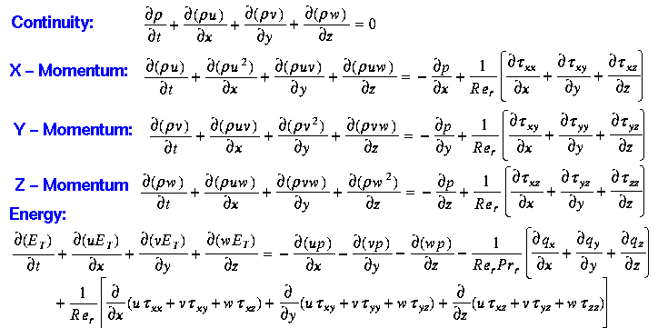
Figure 4 – Navier-Stokes equations, taken from the NASA page
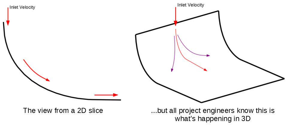
At least, for the source terms, pressure is the one which commonly has the largest impact on the overall flow field. An example of this effect is shown in the figure below. The figure at left is what you would see in a 2D cut – and that’s what we see in the airfoil streamline figures above – but it is not the full story. Whereas the primary effect we see in this section is the the flow turns 90 degrees between the inlet and outlet, there is a notable secondary component here. The increase in static pressure at the wall, which is generated in order to turn the flow translates into a net pressure gradient in the direction into the page as well. In the figure at right, the purple lines are illustrations of the streamlines which arise just because of this directional coupling effect of pressure. Of course, this effect is happening whenever you see a 2D figure of flow turning (whether intended or not), and is part of the explanation for wingtip vortices.
Figure 4
Using the Model
This way of thinking about the flow around an airfoil (or any body) allows one to make useful predictions about how changes to the geometry and operating conditions will impact loads on the body, and to develop an intuition about the static pressure field around the body. This is a working model (whereas almost all other descriptions of airfoil aerodynamics don’t address the static pressure generation mechanism with enough detail or correctness to make predictions) because it allows us to understand what happens when we apply design or operating condition changes to the situation. What happens if the air velocity over the airfoil increases? To the extent that the streamlines stay the same and the flow attached, the pressure gradients have to increase to allow faster air packets to traverse the same streamlines – more exaggerated pressure gradients lead to greater lift. What happens if we curve the airfoil a bit more and turn the flow more (for example, decrease r3 in the Figure 4 above)? The pressure gradient must get steeper in order to turn an air packet on this tighter radius for the same speed, and thus we get more lift again. This breaks down when, at some point, you ask the flow to make a turn that it is unable to do, and you get separated flow. But even then, the same kind of streamline analysis is useful in understanding whats happening.